Gravitational Waves. An Invitation

Albert Einstein originally predicted the existence of gravitational waves in 1916, on the basis of his theory of general relativity. General relativity interprets gravity as a geometric property of spacetime. Einstein also predicted that events in the cosmos would cause ‘ripples’ in spacetime. These ripples are distortions of spacetime itself, which would spread outward, although they would be so minuscule that they would be nearly impossible to detect by any technology foreseen at that time.

The first direct observation of gravitational waves was made on September 14, 2015 and was announced by LIGO (4-kilometer-long interferometers in the United States) and Virgo (3-kilometer-long detector in Italy) in 2016. Previously, gravitational waves had only been inferred indirectly, via their effect on the timing of pulsars in binary star systems. The waveform, detected by both LIGO observatories, matched the predictions of general relativity for a gravitational wave emanating from the inward spiral and merger of a pair of black holes of around 36 and 29 solar masses and the subsequent ‘ringdown’ of the single resulting black hole.

Recently, researchers have detected a signal from what may be the most massive black hole merger yet observed in gravitational waves. The product of the merger is the first clear detection of an ‘intermediate-mass’ black hole, with a mass between 100 and 1.000 times that of the sun. They detected the signal (labeled as GW190521), on May 21, 2019 at LIGO.

The signal, resembling about four short wiggles, is extremely brief in duration, lasting less than one-tenth of a second. From what the researchers can tell, GW190521 was generated by a source that is roughly 5 gigaparsecs away, when the universe was about half its age, making it one of the most distant gravitational-wave sources detected so far.

Many people, with all kinds of backgrounds, are currently talking and discussing this recent event. Many wonder how exactly this is possible and how exactly Einstein already knew what was going on out there in the seemingly infinite space. This blog serves as a stimulation for the curious minded. I tried to keep it short and simple. If there is anything more fascinating than these unbelievable mysterious objects that shake our space and time, then it is the human ability to think about such things. Predicting them, measuring them and hopefully using them for good.

Introduction

There are three essential parts when it comes to any kind of radiation. Here we will formulate it for gravitational radiation. The parts are:

Find and solve a source free equation.
Detection: How do waves influence matter?
Creation: How does matter create waves?

The first point needs a solution of the Einstein equations without sources. To be more precise we want to find a source free wave equation, because they are capable of transmitting energy through a region where there are no sources. In this part we will use a lot of approximations, which are totally fine, since gravitational waves are being originated at events very very far from us. By the time they reach us, they are propagating as a solution of Einstein equations with zero source.

The second point means solving the geodesic equation in the geometry found within the first point. Here we can again use approximations due to the very small amplitudes of the waves reaching us.

The third point asks for solving Einstein’s equations with source.

Find and solve a source free equation.

For the first part we need to linearize general relativity in a similar fashion how it is usually done to get the Newtonian Limit ¹. In this case we can not assume a static approximation because a static approximation does simply not make sense for waves, since we have intrinsically time dependence. So one starts with a flat geometry (often called the background) with small fluctuations depending on $x^\mu$

g_{\mu \nu}\simeq \eta_{\mu \nu}+h_{\mu \nu}(x) + \mathcal{O}(h_{\mu \nu}(x)^2)

The inverse metric is given as

g^{\mu \nu}\simeq\eta^{\mu \nu}-\eta^{\mu \alpha} \eta^{\nu \beta} h_{\alpha \beta}(x) + \mathcal{O}(h_{\mu \nu}(x)^2)

with $\left\|h_{\mu \nu}\right\| \ll 1$ . Next we insert this metric into the source free Einstein equations $R_{\mu \nu}$ in trace-reverse form to find an expression for $\eta_{\mu \nu}(x)$ ².

Why is the last equation considered as the inverse?

Notice that to ensure $g_{\lambda \mu} g^{\mu \nu}=\delta_{\lambda}^{\nu}$ , for a small perturbation $h_{\mu \nu}$ with $\left\|h_{\mu \nu}\right\| \ll 1,$ follows:

\begin{aligned} g_{\lambda \mu} g^{\mu \nu} &=\left(\eta_{\lambda \mu}+h_{\lambda \mu}\right)\left(\eta^{\mu \nu}-\eta^{\mu \alpha} \eta^{\nu \beta} h_{\alpha \beta}\right)=\eta_{\lambda \mu} \eta^{\mu \nu}-\eta_{\lambda \mu} \eta^{\mu \alpha} \eta^{\nu \beta} h_{\alpha \beta}+\eta^{\mu \nu} h_{\lambda \mu}+O\left(h^{2}\right) \\ &=\delta_{\lambda}^{\nu}-\delta_{\lambda}^{\alpha} \eta^{\nu \beta} h_{\alpha \beta}+\eta^{\mu \nu} h_{\lambda \mu}=\delta_{\lambda}^{\nu}-\eta^{\nu \beta} h_{\lambda \beta}+\eta^{\mu \nu} h_{\lambda \mu}=\delta_{\lambda}^{\nu} \end{aligned}

ignoring $\mathcal{O}(h^2)$ and higher.

Let’s calculate the Christoffel symbols

\Gamma_{\alpha \beta}^{\rho}=\frac{1}{2} \eta^{\rho \sigma}\left(\partial_{\alpha} h_{\beta \sigma}+\partial_{\beta} h_{\sigma \alpha}-\partial_{\sigma} h_{\alpha \beta}\right)

since $\partial_{\lambda} \eta_{\mu \nu}=0$ and we are neglecting again terms of order $\mathcal{O}\left(h^{2}\right) .$

The Riemann curvature tensor is

R_{\mu \sigma \nu}^{\rho}=\partial_{\sigma} \Gamma_{\nu \mu}^{\rho}-\partial_{\nu} \Gamma_{\sigma \mu}^{\rho}+\Gamma_{\sigma \lambda}^{\rho} \Gamma_{\nu \mu}^{\lambda}-\Gamma_{\nu \lambda}^{\rho} \Gamma_{\sigma \mu}^{\lambda}

where the last two terms can be ignored because they are $\mathcal{O}\left(h^{2}\right) .$

The Ricci tensor then becomes

\begin{aligned} R_{\mu \nu}\equiv R_{\mu \rho \nu}^{\rho} &=\partial_{\rho} \Gamma_{\nu \mu}^{\rho}-\partial_{\nu} \Gamma_{\rho \mu}^{\rho} \\ &=\frac{1}{2} \eta^{\rho \sigma}\left[\partial_{\rho} \partial_{\nu} h_{\mu \sigma}+\partial_{\rho} \partial_{\mu} h_{\sigma \nu}-\partial_{\rho} \partial_{\sigma} h_{\nu \mu}-\partial_{\nu} \partial_{\rho} h_{\mu \sigma}-\partial_{\nu} \partial_{\mu} h_{\sigma \rho}+\partial_{\nu} \partial_{\sigma} h_{\rho \mu}\right] \\ &=\frac{1}{2} \eta^{\rho \sigma}\left[\partial_{\rho} \partial_{\mu} h_{\sigma \nu}-\partial_{\rho} \partial_{\sigma} h_{\nu \mu}-\partial_{\nu} \partial_{\mu} h_{\sigma \rho}+\partial_{\nu} \partial_{\sigma} h_{\rho \mu}\right] \end{aligned}

We can now define $V_{\mu}\equiv \partial_{\rho} h_{\mu}^{\rho}-\frac{1}{2} \partial_{\mu} h_{\rho}^{\rho}$ and thus the partial derivative reads $\partial_{\nu} V_{\mu}=\partial_{\nu} \partial_{\rho} h_{\mu}^{\rho}-\frac{1}{2} \partial_{\nu} \partial_{\mu} h_{\rho}^{\rho}$ where $h_{\rho}^{\rho}$ is the trace.

With the definition $\square \equiv \partial_{\rho} \partial^{\rho}$ which is $\partial_{\rho} \partial^{\rho}=-\frac{\partial^{2}}{\partial t^{2}}+\vec{\nabla}^{2}$ one gets

R_{\mu \nu}=\frac{1}{2}\left[-\square h_{\mu \nu}+\partial_{\mu} V_{\nu}+\partial_{\nu} V_{\mu}\right]=0

for the Ricci tensor. This looks like a kind of wave equation with some extra chunk. But we can do better. Gauge freedom allows, despite the fact that we had to choose certain coordinates such that $g_{\mu \nu}=\eta_{\mu \nu}+h_{\mu \nu}$ , to make coordinate changes which preserves $\eta_{\mu \nu}$ , but will generally change the form of $h_{\mu \nu}(x)$ .

If one transforms $x^{\mu} \rightarrow x^{\mu^{\prime}}=x^{\mu}+\delta^{\mu}(x)$ , which preserves our form of the metric as a flat backgroud + fluctuations with a small $\delta^{\mu}$ . Recall that the metric changes under coordinate transformations as usual

g_{\mu \nu} \rightarrow g_{\mu^{\prime} \nu^{\prime}}=\frac{\partial x^{\mu}}{\partial x^{\mu^{\prime}}} \frac{\partial x^{\nu}}{\partial x^{\nu^{\prime}}} g_{\mu \nu}

So we get

g_{\mu \nu}=\eta_{\mu \nu}+h_{\mu \nu} \rightarrow g_{\mu^{\prime} \nu^{\prime}}=\eta_{\mu \nu}+\underbrace{h_{\mu \nu}-\partial_{\mu} \delta_{\nu}-\partial_{\nu} \delta_{\mu}}_{h_{\mu^{\prime} \nu^{\prime}}}

where $\delta_{\mu}=\eta_{\mu \nu} \delta^{\nu}$ .

Now we can compare $h_{\mu \nu} \rightarrow h_{\mu \nu}^{\prime}=h_{\mu \nu}-\partial_{\mu} \delta_{\nu}-\partial_{\nu} \delta_{\mu}$ with $A_{\mu} \rightarrow A_{\mu}^{\prime}=A_{\mu}-\partial_{\mu} \Phi$ which we know from electromagnetism. The form of the first equation is very similar to the second one, but taking care that the ‘potential’ has two indices instead of one. A useful aspect of Gauge freedom is that the physical degrees of freedom do not change. In this case, the physical curvature $R_{\nu \lambda \rho}^{\mu}$ is unchanged so that solutions to $R_{\mu \nu}=0$ remain solutions. Here, one can use a gauge so that $V_{\mu} \rightarrow V_{\mu}^{\prime}=\partial_{\alpha} h_{\mu}^{\alpha}-\frac{1}{2} \partial_{\mu} h_{\alpha}^{\alpha}=0 .$

From $R_{\mu \nu}=-\frac{1}{2} \square h_{\mu \nu}=0$ follows that $\square h_{\mu \nu}=0$ .

So we finally found

\square h_{\mu \nu}=0

which is a wave equation, so we we can immediately write down a plane wave solution.

Let’s make the usual Ansatz

h_{\mu \nu}=a_{\mu \nu} e^{i k_{\lambda} x^{\lambda}}

where one can think of $a_{\mu \nu}$ as the polarization and the amplitude of the wave. Feeding this into $\square h_{\mu \nu}=$ $-k_{\lambda} k^{\lambda} h_{\mu \nu}=0$ gives $k_{\lambda} k^{\lambda}=0$ since $h_{\mu \nu}=0$ is a solution but not a very interesting one. Thus $k^{\lambda}$ is a null vector, and one can write it as $k^{\lambda}=(|\vec{k}|, \vec{k})$ with $k_{\lambda} k^{\lambda}=-|\vec{k}|^{2}+\vec{k} \cdot \vec{k}=0 .$ With the frequency $\omega=|\vec{k}|$ and the wavelength $\lambda=\frac{2 \pi}{\omega}$ the wave travels with phase velocity $v=\lambda \frac{\omega}{2 \pi}=1$ in the direction $\vec{k}$ . Thus, the gravitational wave travels with the speed of light as one would expect because the gravitational fluctuations are massless.

The symmetric $4 \times 4$ matrix (10 independent components) $a_{\mu \nu}$ describes amplitude and polarization of the wave and can be simplified because using any $\delta_{\mu}$ so that $\square \delta_{\mu}=0$ these four functions can be used to make any four components of $h_{\mu \nu}$ vanish identically (Residual gauge freedom). Choosing $h_{t i}=0$ (3 degrees of freedom) and $h_{\mu}^{\mu}=0$ (traceless) (1 degree of freedom) or $a_{t i}=0$ and $a_{\mu}^{\mu}=0$ represents three plus one terms such that the ten degrees of freedom of the symmetric matrix $a_{\mu \nu}$ are reduced to six independent components. With the previous gauge condition $V_{\mu}$ follows

\begin{array}{ll} V_{t}=\partial_{\rho} h^{\rho}{ }_{t}-\frac{1}{2} \partial_{t} h_{\rho}^{\rho}=\partial_{t} h_{t}^{t}=i \omega a_{t t} e^{i k_{\lambda} x^{\lambda}}=0 & \Rightarrow \quad a_{t t}=0\\ V_{i}=\partial_{\rho} h_{i}^{\rho}-\frac{1}{2} \partial_{i} h_{\rho}^{\rho}=\partial_{j} h_{i}^{i}=i k_{j} a_{j i} e^{i k_{\lambda} x^{\lambda}}=0 & \Rightarrow \quad k^ja_{j i}=0 \\ \end{array}

where the equation $k^{j} a_{j i}=0$ means that the waves are transverse or, in other words, that the spatial wave vector $\vec{k}$ is ‘perpendicular’ to the polarization tensor. If the wave vector is chosen to be $k^{\mu}=(\omega, 0,0, \omega)$ with the spatial part $\vec{k}=(0,0, \omega)$ then $a_{z i}=0$ follows from the transversality condition. Thus only two independent components of $a_{\mu \nu}v$ remain which are $a_{x x}=-a_{y y}($ traceless $)$ and $a_{x y}=a_{y x}$ (symmetric). This additional choice is called transverse-traceless gauge, and

h_{\mu \nu}(x)=\left(\begin{array}{cccc} 0 & 0 & 0 & 0 \\ 0 & a & b & 0 \\ 0 & b & -a & 0 \\ 0 & 0 & 0 & 0 \end{array}\right) e^{i k_{\lambda} x^{\lambda}}

is the final form of $h_{\mu \nu}(x) .$

In the linearized theory one gets more general solutions by adding solutions of this form. This is, however, not possible in the full-blown version of general relativity which is highly non-linear. So, the part of finding a source free wave equation is done.

Detection: How do waves influence matter?

The next part is the detection of gravitational waves. With the metric solution $g_{\mu \nu}=\eta_{\mu \nu}+h_{\mu \nu}(x)$ where $\eta_{\mu \nu}$ is flat spacetime and $h_{\mu \nu}(x)$ is defined in our last equation. We can now explore how test particles respond to this time-dependent geometry using the geodesic equation

\frac{d^{2} x^{\mu}}{d \lambda^{2}}+\Gamma_{\alpha \beta}^{\mu} \frac{d x^{\alpha}}{d \lambda} \frac{d x^{\beta}}{d \lambda}=0 \quad \Rightarrow \quad \frac{d U^{\mu}}{d \tau}+\Gamma_{\alpha \beta}^{\mu} U^{\alpha} U^{\beta}=0 \quad \Rightarrow \quad \frac{d U^{\mu}}{d \tau}=-\Gamma_{\alpha \beta}^{\mu} U^{\alpha} U^{\beta}

for timelike and $U^{\mu}=\frac{d x^{\mu}}{d \tau} .$ If the particle is at rest for $\tau=0$ such that $U^{\mu}(0)=(1,0,0,0)$ then

\frac{d U^{\mu}}{d \tau}(0)=-\Gamma_{00}^{\mu}=-\frac{1}{2} \eta^{\rho \sigma}\left(\partial_{0} h_{\sigma 0}+\partial_{0} h_{0 \sigma}-\partial_{\sigma} h_{00}\right)=0

since $h_{t i}=h_{t t}=0$ and this means that if the particle begins at rest, it remains at rest as the wave passes! However, this is just a statement that the coordinate position of the mass is unchanged because the particle is at rest and the acceleration is zero. Thus, maybe two test masses and the distance between them show an effect.

Actually, one could have anticipated the need for at least two particles from the equivalence principle. Observing only one particle does not allow to distinguish whether the lab is in the gravitational field of the earth or being accelerated. Only if one observes two particles one can detect tidal forces because the two particles come closer because they move towards the center of the earth while in the case of acceleration they move on parallel paths and keep the distance they initially had. Detecting curvature is impossible with only one test mass because one can always find coordinates in which the particle is and stays at rest. With two test masses one can see whether the distance between them remains constant or not.

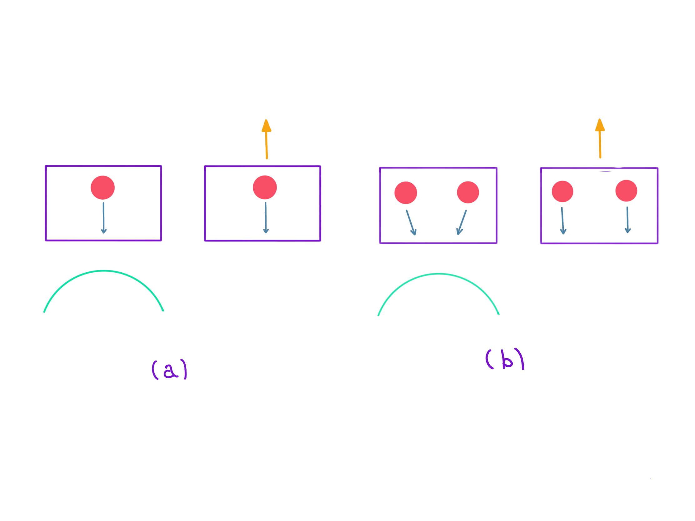
Observing only one particle does not allow to distinguish whether the lab is in a gravitational field or being accelerated (a) vs. observing two particle does allow to distinguish whether the lab is in a gravitational field or being accelerated due to geodesic deviation (b). (Fig. 1)

For one mass at the spatial coordinate (0,0,0) and another mass at spatial coordinate $(\varepsilon, 0,0)$ one finds for the distance

\begin{aligned} \int \sqrt{d s^{2}} &=\int \sqrt{g_{\mu \nu} d x^{\mu} d x^{\nu}}=\int_{0}^{\varepsilon} \sqrt{g_{x x}} d x \\ & \approx \sqrt{g_{x x}(x=0)} \varepsilon=\sqrt{1+h_{x x}(x=0)} \varepsilon \approx\left[1+\frac{1}{2} h_{x x}(x=0)\right] \varepsilon=\left[1+a e^{i k_{\lambda} x^{\lambda}}\right] \varepsilon \end{aligned}

Look! This varies now with time. Despite the fact that one particle remains at $x=0$ and the other at $x=\varepsilon$ , the invariant distance between them changes because this value varies with time. This is the difference between the coordinates and the physical reality. In the chosen coordinates the two masses do not move, but in reality they move with respect to each other.

To get a better idea of what a gravitational wave does, the values $a$ and $b$ in our found expression of $h_{\mu \nu}$ are chosen such that $a$ is small and $b$ is zero, and the wave travels along the $z$ -axis. This gives

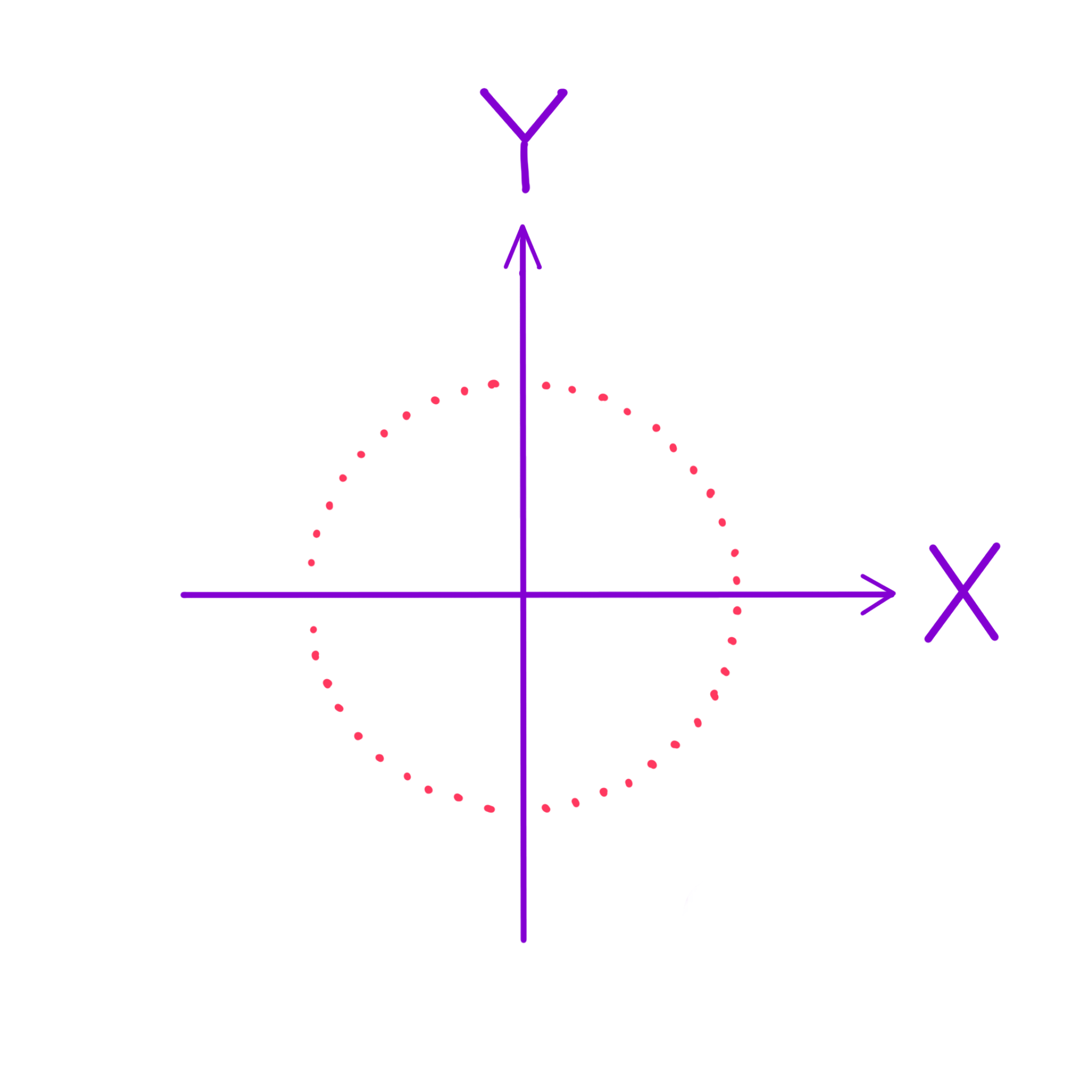
h_{\mu \nu}(x)=\left(\begin{array}{cccc} 0 & 0 & 0 & 0 \\ 0 & a & 0 & 0 \\ 0 & 0 & -a & 0 \\ 0 & 0 & 0 & 0 \end{array}\right) \sin (k z-\omega t)

for the real part. A system of masses is set up in the $x y$ -plane at $z=0$ such that one mass is at the center and the others build a ring around it. The gravitational wave comes along the $z$ -axis perpendicular to the $x y$ -plane. The metric at $z=0$ is

\left.d s^{2}\right|_{z=0}=-d t^{2}+\big[1-a \sin (\omega t)\big]\, d x^{2}+\big[1+a \sin (\omega t)\big]\, d y^{2}

and with $X=\left(1-\frac{1}{2} a \sin (\omega t)\right) x$ and $Y=\left(1+\frac{1}{2} a \sin (\omega t)\right) y$ the metric becomes

\left.d s^{2}\right|_{z=0}=-d t^{2}+d X^{2}+d Y^{2}

plus terms of order $\mathcal{O}\left(a^{2}\right) .$ This is now flat Minkowski space, and one can visualize the geometry with Euclidean intuition. The scenario for the test particle can now be illustrated as in (Fig. 2).

The ring of test particle lies in the X-Y-plane – The gravitational wave passes through the particles along a line perpendicular to the plane of the particles, i.e. following the observer's line of vision into the screen. (Fig. 2)

The result is called the plus-polarization (+ polarization) presented in (Fig. 3(a)).

If one instead chooses the values $a$ and $b$ such that $b$ is small and $a$ is zero, while the wave still travels along the $z$ -axis, the real part of the perturbation of the metric is

h_{\mu \nu}(x)=\left(\begin{array}{llll} 0 & 0 & 0 & 0 \\ 0 & 0 & b & 0 \\ 0 & b & 0 & 0 \\ 0 & 0 & 0 & 0 \end{array}\right) \sin (k z-\omega t)

and corresponds to

\left.d s^{2}\right|_{z=0}=-d t^{2}+d x^{2}+2 b \sin (\omega t)\; d x\; d y+d y^{2}

for the distance. With $X=x+\frac{1}{2} b \sin (\omega t) \;y$ and $Y=y+\frac{1}{2} b \sin (\omega t) \;x$ the metric becomes

\left.d s^{2}\right|_{z=0}=-d t^{2}+d X^{2}+d Y^{2}

because $d X=d x+\frac{1}{2} b \sin (\omega t) \;d y$ and $d Y=d y+\frac{1}{2} b \sin (\omega t)\; d x$ as well as $d X^{2} \approx d x^{2}+b \sin (\omega t)\; d x\; d y$ and $d Y^{2} \approx d y^{2}+b \sin (\omega t) \;d x\; d y .$ This is again flat Minkowski space, and the result is called the cross-polarization ( $\times$ polarization $)$ shown in (Fig. 3(b)).

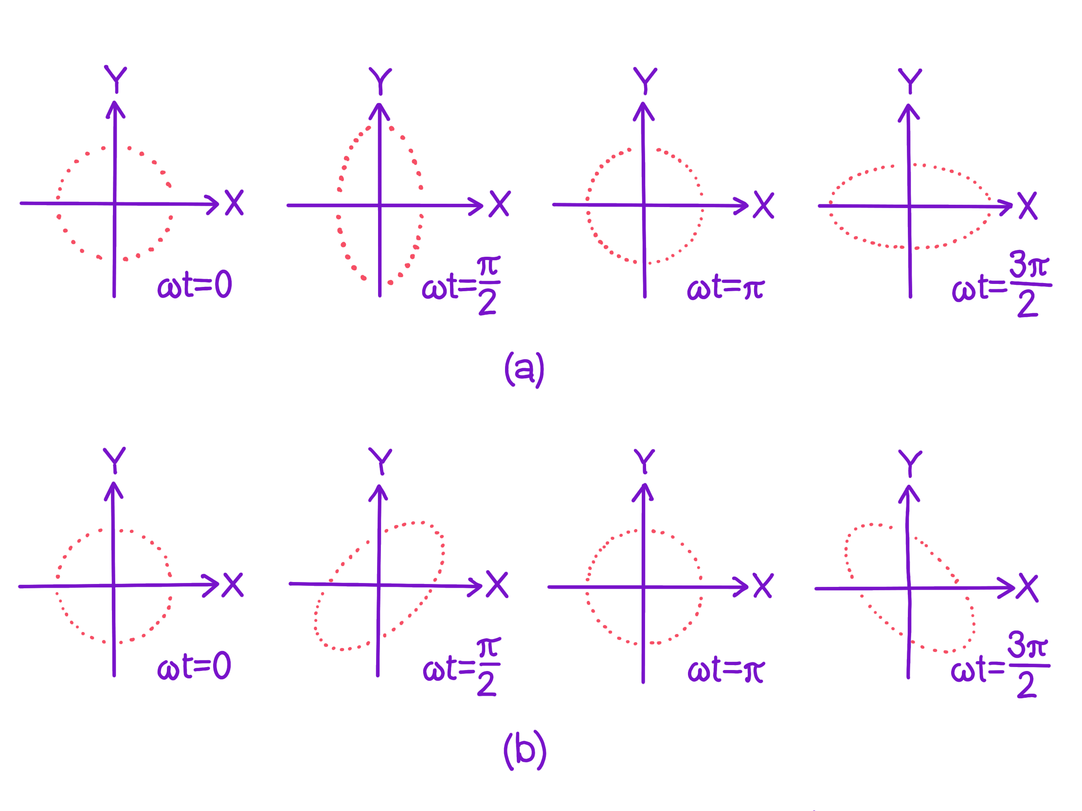
Polarization of the gravitational wave – The effect of a plus-polarized gravitational wave on a ring of particles (a). The effect of a cross-polarized gravitational wave on a ring of particles (b). (Fig. 3)

These are the two independent polarization states of the plane gravitational wave. The polarization of the electromagnetic wave can similarly be decomposed into an $x$ -polarization and a $y$ -polarization. The difference though is that the electromagnetic wave is invariant if one flips it by $180^{\circ}$ while the gravitational wave is invariant if one flips it by $90^{\circ} .$ One can tie that to the fact that the graviton has spin two and the photon has spin one.

To really detect gravitational waves one could use several such rings of masses because one does not know the direction in which the wave comes and the ring should be perpendicular to this direction. With a ruler one could measure how the ring changes. The ruler does not expand and contract the same way because the above analysis used the geodesic equation for free test particles, and the atoms building the ruler are not free but also experience electromagnetic binding forces which swamp the gravitational distortion. Tiny displacement in physics are not measured with rulers but with interferometers.

The LIGO (Laser Interferometer Gravitational-Wave Observatory) uses four kilometer long Michelson interferometers with mirrors attached to free test masses which are actually hanging but are free to swing. The accuracy is in the order of $10^{-21}$ and the change of length is in the order of $10^{-18}\; \mathrm{m} .$ So much noise has to be eliminated that quantum fluctuations must be filtered out. There are other projects planned. The LISA (Laser Interferometer Space Antenna) project uses satellites in space with a length scale for the arms of $5 \cdot 10^{6}\; \mathrm{km},$ and the PTR (Pulsar Timing Arrays) will observe irregularities in what should be periodic signals from pulsars.

Creation: How does matter create waves?

The last question related to gravitational waves is how they get created. Thus one has to solve Einstein’s equations in the presence of sources, and one cannot use small approximations because one wants to see a signal big enough to be measured. One can create electromagnetic waves by moving charges as in an antenna to get uniform radiation, but for gravitational wave production there is nothing popping energy into the system to make it steady state. One has a time-dependent system which produces the radiation. If two black holes come close then they merge and become a single black hole. Such an event has been observed by LIGO. Studying realistic gravity wave generation is difficult and will not be shown here, but there are two interesting features. One is the possibility of multipole expansion and the other is the observable signals from the binary mergers of two black holes.

Firstly, just like any other form of radiation, one can take the far field limit and do a multipole expansion of the power distribution. For both electromagnetic and gravitational waves, the monopole contribution vanishes because of conservation of charge and mass. The leading electromagnetic term is dipole. For General Relativity, however, also the dipole term vanishes because of conservation of angular momentum and the ability to coordinatize to zero the center of mass motion. Thus the lowest term is quadropole. Secondly, appreciable signals can arise from binary mergers. In particular, when massive black holes merge they can release gravitational wave energies in the order of the mass of the sun. To analyze a merger, the problem is often broken up into stages. Everything could in principle be done numerically, but Einstein’s equations are hard and one would have to simulate over a large region to get far-field behavior.

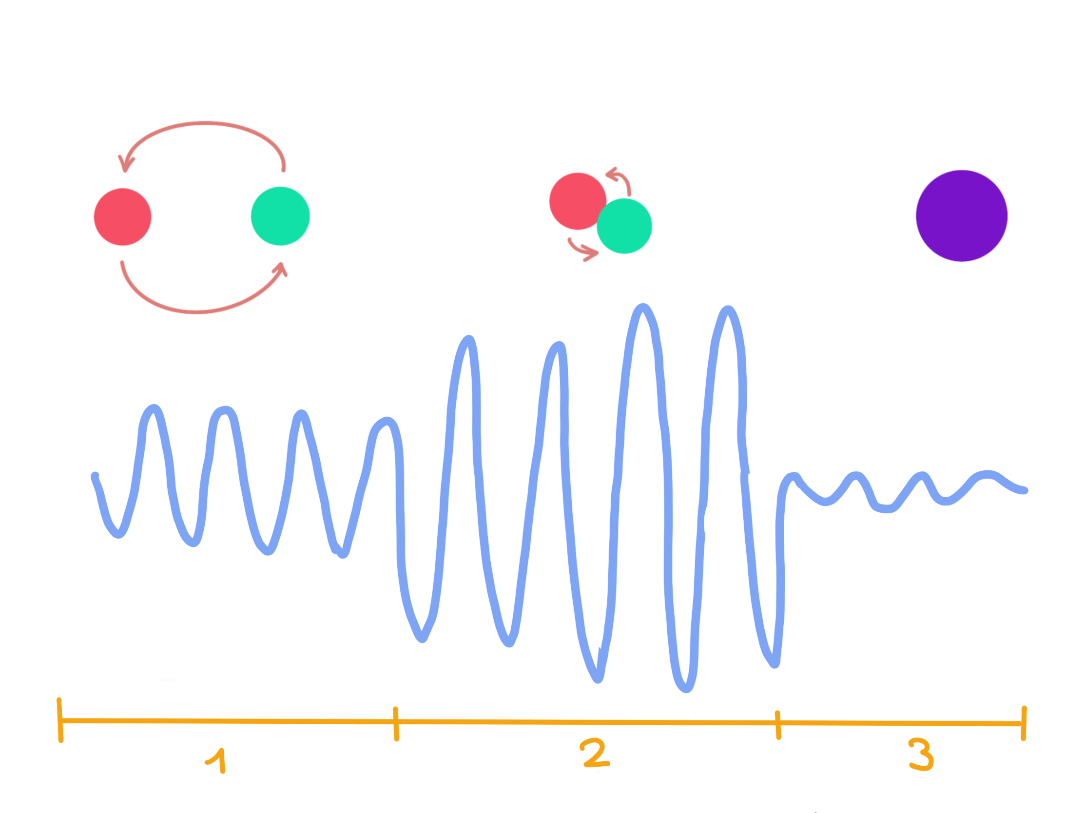
Two black holes merge in three phases. The first phase is called inspiral, and one can use post-Newtonian approximations (linear approximations) to address the two-body problem. The second phase is called merger, and one uses numerical calculations to handle it. The third and last phase is called ringdown where the resulting black hole still wobbles before it settles down to a Kerr black hole, and one uses single-body black hole perturbation theory for calculations.

One of the fascinating things about black hole mergers compared to other merger events is the ringdown signature, since ringdown only happens for black holes, its observation is a direct observation of black holes.

*The 'chirp' characteristic of a typical black hole merge - Polarization of the gravitational wave – Inspiral phase (1), merge phase (2) and the ringdown (3). (Fig. 4)*

Apart from my self-made illustration, there are some pretty neat simulations on YouTube, such as this one:

References

Spacetime and Geometry: An Introduction to General Relativity by Sean Carroll.
General Relativity by Rober M. Wald.
Gravitational Waves: Volume I: Theory and Experiments by Michele Maggiore.
Gravitational Waves: Volume II: Astrophysical Sources by Michele Maggiore.
Elements of General Relativity by Piotr T. Chrusciel.

This is often called post-Newtonian approximation in gravitational physics.↩
If you want to make your life even harder, you can also choose a much more complicated geometry. For example, one could replace $\eta$ with the Schwarzschild Metric or a suitable metric to model a cosmological scenario. But that is left as an exercise to you.↩

← Previous post

The Last Frontier

Pages

Blog Posts

Gravitational Waves - An Invitation